
A DEATHCON Thrunting Workshop Overview Part 5: Model-Assisted Threat Hunting (M-ATH)
Machine learning, statistics, and HTTP events…oh my!

If you’re just tuning in now, welcome! This is part 5 of a series on a workshop previously given at DEATHCon 2024. If you want to start from the beginning, head over here.
Introduction: Model-Assisted Threat Hunting (M-ATH)
Welcome to Part 5 of the DEATHCON Thrunting Workshop, where we dive into Model-Assisted Threat Hunting (M-ATH)! Because who doesn't love a bit of machine learning (ML) magic to spice up their threat hunting?

WHOA, not that spice.
In this post, we'll use Splunk's built-in ML capabilities to uncover threats hiding within HTTP traffic. By using techniques like anomaly detection and clustering, ML can transform overwhelming log data into actionable insights.
Are you ready to uncover the signal in the noise? Let’s thrunt!

Prepare Phase - Understanding M-ATH
M-ATH leverages ML to automate and enhance the threat hunting process. Its techniques help identify subtle patterns of malicious behavior that might evade manual analysis in high-volume and complex datasets like network traffic. These techniques increase accuracy, efficiency, and adaptability in your hunting! Thrunt better!
Why Use ML for Traffic Analysis?
Can process MASSIVE amounts of HTTP traffic data efficiently
Identifies patterns that human analysts might miss
Reduces false positives through statistical validation
Adapts to changing traffic patterns over time
Different Levels of M-ATH
M-ATH has many levels, ranging from basic pattern recognition to advanced data science techniques. For now…we will stick to the basics. Think of it as an introduction, where we are only scratching the surface of ML. But hey, you have to start somewhere, right?
If you're interested in digging deeper into the data science aspects (which are rad and things we may cover in the future), Splunk offers two powerful apps that can help:
🔹 Splunk Machine Learning Toolkit (MLTK): Pre-built ML algorithms for supervised, unsupervised, and time series analysis
🔹 Splunk Deep Science and Deep Learning (DSDL): Extends MLTK, integrating custom ML & deep learning models using tools like Jupyter notebooks

Splunk Commands We'll Use
In this workshop, we'll leverage built-in SPL commands to apply ML techniques like clustering, anomaly detection, and statistical outlier identification. Yes, you can do ML right in the search bar in Splunk!
Key Commands:
anomalydetection - Detect unusual patterns automatically
kmeans - Group similar events using clustering
stats - Calculates aggregate statistics
bin - Bucket numerical data into ranges for easy analysis
eventstats - Add summary statistics to individual events
Techniques We'll Use
Anomaly Detection: Finding statistical outliers in traffic patterns
Clustering: Grouping similar traffic behaviors
Statistical Analysis: Identifying significant deviations
Data Visualization: 3D plotting of traffic characteristics
Hypothesis
Attackers are exploiting long-duration HTTP connections to exfiltrate sensitive data from the network. Advanced analytical methods will enable us to detect these anomalous sessions by examining patterns in session duration, data transfer volumes, and time-based features.
Common Data Exfiltration Indicators
Unusually long session durations
High volume of outbound traffic
Anomalous traffic patterns
Statistical outliers in data transfer sizes
Unusual timing or frequency of connections
Step 1: Data Wrangling and Preparation
Why this step?
Before applying ML techniques, we need to properly prepare our data.
Remember: 🗑️ Garbage In = Garbage Out.

If you’re already using Splunk's search commands effectively, you’re probably preprocessing your data without realizing it!
Key Data Preparation Tasks (many using standard SPL!):
Verify that categorical data is properly encoded
Check that timestamps are in a consistent format
Confirm calculated fields have meaningful values
Look for any obvious data quality issues
Example SPL for Data Preparation
Convert HTTP methods to numerical values (categorical encoding):
| eval http_method_encoded = case(

http_method="GET", 1,

http_method="POST", 2,

http_method="PUT", 3,

http_method="DELETE", 4,

http_method="HEAD", 5,

1=1, 0)
Standardize timestamps to enable analysis of changes over time:
| eval firstTime=strftime(firstTime,"%Y-%m-%d %H:%M:%S")

| eval lastTime=strftime(lastTime,"%Y-%m-%d %H:%M:%S")
Create time-based bins for analysis:
| bin _time span=1hFeature engineering with session metrics:
| eval session_duration=lastTime - firstTime

| eval bytes_ratio=bytes_out/bytes_in

| eval traffic_volume=bytes_in + bytes_out
Leading to Step 2:
With our data properly prepared using these common SPL commands (which perform the same as traditional ML preprocessing steps!), we can visualize top traffic sources and begin our anomaly detection analysis. The standardized formats and engineered features we've created will ensure our ML techniques can effectively identify sus 🚩 patterns in the data.
Step 2: Visualizing Top Traffic Sources
Why this step? Before diving into advanced ML techniques, we need to understand the basic distribution of our HTTP traffic. This step helps us:
Establish a baseline for normal traffic volumes
Identify top traffic sources that might skew our analysis
Spot obvious anomalies before applying ML techniques (Errors that we may need to throw out or even actual bad. You never know.)
Create a foundation for more sophisticated pattern analysis
Understanding Traffic Distribution
Total traffic from combined inbound and outbound bytes helps identify high-volume sources
Relationship between bytes_in and bytes_out can indicate data exfiltration
How traffic is distributed across different IPs
Distribution of Traffic Query:
index=thrunt sourcetype=stream:http

# Aggregate total requests, inbound, and outbound traffic per source IP
| stats
    sum(bytes_in) as bytes_in,   # Total inbound data
    sum(bytes_out) as bytes_out,  # Total outbound data
    count as total_requests       # Number of requests
    by src_ip

# Calculate total traffic (sum of inbound and outbound bytes)
| eval total_traffic = bytes_in + bytes_out

# Compute traffic ratio (outbound vs. inbound)
| eval traffic_ratio = bytes_out / bytes_in

# Sort results by highest total traffic
| sort -total_traffic

# Show only the top 10 highest-traffic source IPs
| head 10

# Organize results in a structured table
| table src_ip total_requests bytes_in bytes_out total_traffic traffic_ratio
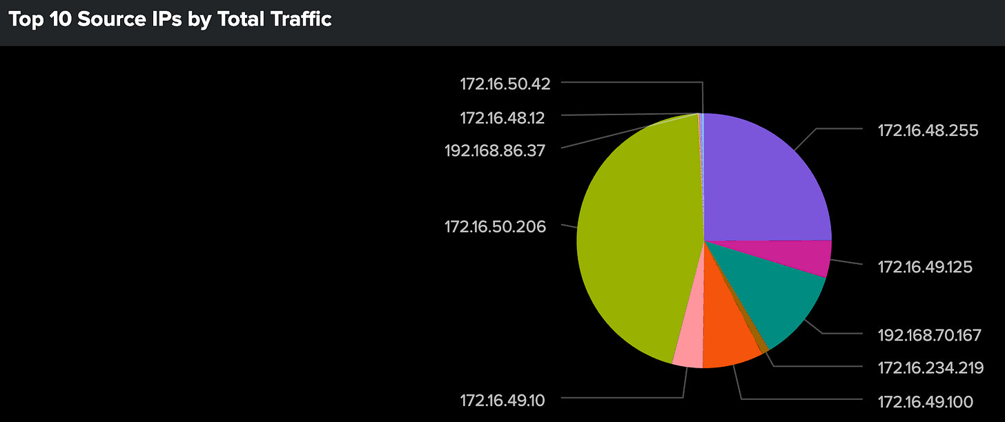
Analyzing the Results:
Look for sources with disproportionate traffic volumes
Identify unusual ratios between ingress and egress traffic
Note sources with high request counts but low traffic volumes (or vice versa)
Compare traffic patterns against known normal behavior (use your baseline hunting findings!)
Flag any sources that appear anomalous for deeper investigation (escalate to your incident response teams!)
Key Questions to Ask:
Do any sources stand out with unusually high traffic?
Are there sources with suspicious inbound/outbound ratios (remember that feature engineering we did!)?
How does the traffic distribution compare to normal patterns (baseline)?
Are there any unexpected sources in the top 10?
Leading to Step 3:
Now that we understand normal, we can look for deviations. The baseline we've established here will help us understand which traffic patterns truly deserve attention when we apply our anomaly detection techniques in the next step.
What to Watch For:
Sources appearing in top traffic that shouldn't be there
Unusual spikes in traffic volume
Patterns that don't align with business hours
Sources with abnormal bytes_out to bytes_in ratios
Step 3: Filtering for Long-Duration HTTP Traffic
Why this step? Long-duration HTTP sessions often indicate suspicious activity. Most legitimate web traffic consists of short, discrete requests. Extended sessions could suggest:
Data exfiltration attempts
Command and control (C2) channels
Unauthorized file transfers
Beaconing behavior
Key Duration Analysis Concepts:
Session Duration: Check the time between first and last seen traffic
Data Volume: Amount of data transferred during the session
Traffic Patterns: How data flows over the session duration
Time-of-Day Analysis: When long sessions occur in your environment
Filtering Duration Query:
index=thrunt sourcetype=stream:http

# Aggregate HTTP session data per unique session
| stats
    count,
    min(_time) as firstTime,   # Capture session start time
    max(_time) as lastTime,    # Capture session end time
    sum(bytes_in) as bytes_in,  # Total inbound data
    sum(bytes_out) as bytes_out  # Total outbound data
    by url src_ip dest_ip http_user_agent

# Calculate session duration
| eval duration = lastTime - firstTime

# Filter for long-duration sessions (>1 hour) with high outbound traffic (>500KB)
| where duration > 3600 AND bytes_out > 500000

# Format timestamps for better readability
| eval firstTime = strftime(firstTime, "%Y-%m-%d %H:%M:%S")
| eval lastTime = strftime(lastTime, "%Y-%m-%d %H:%M:%S")

# Convert duration to hours for easier interpretation
| eval duration_hours = duration / 3600

# Convert bytes_out to megabytes (MB) for better readability
| eval bytes_out_mb = bytes_out / 1024 / 1024

# Display key session details in a structured table
| table url src_ip dest_ip bytes_out_mb duration_hours firstTime lastTime http_user_agent

# Sort results by longest session duration
| sort -duration_hours
Analyzing the Results:
Examine sessions lasting longer than 1 hour (3600 seconds)
Focus on connections with large outbound data transfers (>500KB)
Look for suspicious URLs or user agent strings
Identify patterns in source/destination IP pairs
Note the timing of these long sessions
Common Red Flags:
Sessions spanning unusual hours (overnight, weekends)
Disproportionate outbound data volume
Generic or suspicious user agent strings
Repeated patterns in connection timing
Connections to unusual or unexpected destinations
Leading to Step 4:
Once we identify our long-duration sessions, we'll use statistical analysis to understand their distribution. This will help us identify truly anomalous patterns rather than legitimate long-running connections. The bin command will help us visualize these patterns more effectively.
Are these durations consistent with legit business activities? (should your HR employees be making outbound file transfers?)
Do the data transfer volumes align with the session durations?
Are there patterns in the timing or frequency of these sessions?
How do these sessions correlate with our top traffic sources from Step 2?
Step 4: Analyzing Duration Distribution with the bin Command
Let’s visualize our HTTP session durations by applying the bin command from our Hypothesis-Driven scenario and creating a histogram. This method uncovers session length patterns that raw data alone fails to reveal.

Refresher
The bin command in Splunk groups continuous numerical values into discrete sets (or bins), making it easier to analyze distributions and identify patterns. In our case, we'll use it to group session durations into one-hour intervals. For more details, refer to the bin command documentation.
bin Query:
index=thrunt sourcetype=stream:http

# Aggregate HTTP session data
| stats
    count,
    min(_time) as firstTime,   # Capture session start time
    max(_time) as lastTime,    # Capture session end time
    sum(bytes_in) as bytes_in,  # Total inbound data
    sum(bytes_out) as bytes_out  # Total outbound data
    by url src_ip dest_ip http_user_agent

# Calculate session duration
| eval duration = lastTime - firstTime

# Filter for long-duration sessions (>1 hour)
| where duration > 3600

# Group session durations into 1-hour bins (3600-second intervals)
| bin duration span=3600

# Count the number of sessions in each duration bin
| stats count by duration

# Sort results to highlight the most common session durations
| sort - count
Key Components of this query:
Groups data into 1-hour (3600-second) intervals
Counts the number of sessions in each duration bin
Sorts results to highlight the most common duration ranges

Analyzing the Histogram
See any of these patterns?
Natural groupings in session durations
Unusual gaps or spikes in the distribution
Sessions that fall far outside the normal distribution
Step 5: Detecting Anomalies with the anomalydetection Command
Why this step? The anomalydetection command helps identify statistical outliers in your data by using probability. It flags unusually small probabilities as sus. This is particularly valuable for threat hunting because it establishes a baseline of normal and then flags deviations for us!
anomalydetection Query:
index=thrunt sourcetype=stream:http

# Select only necessary fields to improve performance
| fields _time url src_ip dest_ip http_user_agent bytes_in bytes_out

# Aggregate session data by unique URL, source IP, destination IP, and user agent
| stats
    count,
    min(_time) as firstTime,  # Capture session start time
    max(_time) as lastTime,   # Capture session end time
    sum(bytes_in) as bytes_in,  # Total inbound data
    sum(bytes_out) as bytes_out  # Total outbound data
    by url src_ip dest_ip http_user_agent

# Calculate session duration
| eval duration = lastTime - firstTime

# Filter for long-duration HTTP sessions (>1 hour)
| where duration > 3600

# Apply anomaly detection to identify statistical outliers
| anomalydetection

# Flag anomalous sessions (isOutlier = 1 if probable_cause is not empty)
| eval isOutlier = if(probable_cause != "", "1", "0")

# Format timestamps for better readability
| eval firstTime = strftime(firstTime, "%Y-%m-%d %H:%M:%S"),
       lastTime = strftime(lastTime, "%Y-%m-%d %H:%M:%S")

# Organize the final output for analysis
| table url src_ip dest_ip http_user_agent firstTime lastTime bytes_in bytes_out duration isOutlier probable_cause
Understanding the SPL:
fields: Select only necessary fields to improve performance
stats: Aggregate data by unique combinations of URL, IP, and user agent
anomalydetection: Identify statistical outliers in the dataset
eval isOutlier: Create binary flag for anomalous events
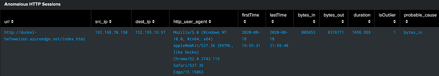
Analyzing the Results:
Focus on events flagged as outliers (isOutlier=1)
Review the probable_cause field to understand why events are anomalous
Look for patterns among anomalous events
Cross-reference with previous findings about long-duration sessions
Leading to Step 5:
Now that we have identified individual anomalies, we will use clustering to group similar sessions and visualize their relationships.
Key Questions to Ask:
Are anomalous sessions correlated with specific source IPs?
Do certain user agents appear more frequently in anomalous traffic?
How do the anomalies cluster together in terms of timing and behavior?
What legitimate business processes might explain some of these anomalies?
Step 6: Clustering HTTP Traffic for Anomaly Detection
We have already identified sessions with unusually long durations and high data transfer volumes. Now, we will use the kmeans command to group these sessions into clusters based on their similarity across three dimensions:
duration (x-axis)
bytes_in (y-axis)
bytes_out (z-axis)
We’re using KMeans clustering because it’s fast, scalable, and effective for our three dimensions of numerical data. Unlike other clustering methods, KMeans lets us define the number of clusters (k), allowing us to group similar sessions while making anomalies stand out visually. In our workshop, we chose three clusters. However, this is just a starting point; we may need to iterate on the cluster number to improve accuracy.
Why Clustering?
Clustering vs. Stacking
Stacking aggregates data by counting and summarizing values across different fields. In contrast, clustering digs into multidimensional spaces (whoa 3D) to reveal hidden patterns and relationships that simple aggregations might miss.
Clustering Query:
index=thrunt sourcetype=stream:http

# Aggregate key metrics per HTTP session
| stats count min(_time) as firstTime max(_time) as lastTime sum(bytes_in) as bytes_in sum(bytes_out) as bytes_out by url src_ip dest_ip http_user_agent

# Calculate session duration
| eval duration=lastTime - firstTime

# Filter for sessions longer than 1 hour (3600 seconds)
| where duration > 3600

# Format timestamps for better readability
| eval firstTime=strftime(firstTime,"%Y-%m-%d %H:%M:%S"), lastTime=strftime(lastTime,"%Y-%m-%d %H:%M:%S")

# Apply K-Means clustering with k=3 on duration, bytes_in, and bytes_out
| kmeans k=3 duration bytes_in bytes_out

# Organize the output for analysis
| table src_ip, dest_ip, http_user_agent, url, duration, firstTime, lastTime, bytes_in, bytes_out, CLUSTERNUM

# Rename fields for clarity in visualization
| rename duration as x, bytes_in as y, bytes_out as z, CLUSTERNUM as clusterId
Visualizing Clusters
The 3D scatter plot will help us analyze these clusters by visually mapping relationships between:
Session duration (x-axis)
Inbound data volume (y-axis)
Outbound data volume (z-axis)
Each point in the plot represents a session, grouped by similarity and colored by the CLUSTERNUM field. This coloring allows us to distinguish (hello, pretty colors🌈) different behavioral groups and spot potential anomalies easily.
What Are We Looking For in This Visualization?
Outliers or separate clusters that indicate unusual behavior:
Clusters with disproportionately high duration (x) and bytes_out (z) may indicate data exfiltration.
Single points far removed from any cluster could represent highly unusual and potentially suspicious activity.
After analyzing this scatter plot, the next steps involve deeper investigation into the outliers and separate clusters. We should examine specific sessions more closely, review associated user behaviors, or correlate these findings with other security events.
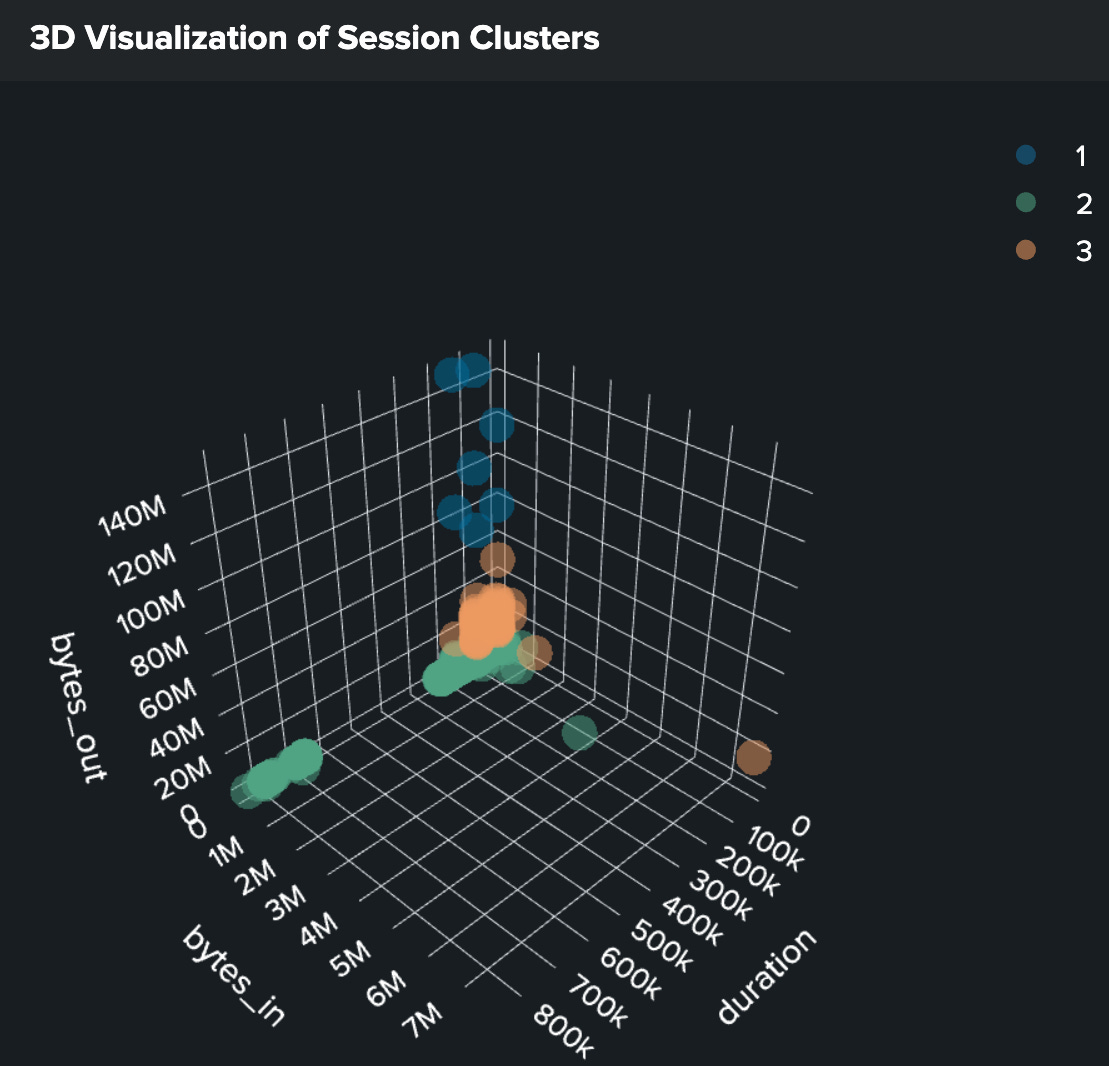
Interpreting the Clusters
When analyzing the clusters, focus on:
Isolated points far from cluster centers (potential anomalies)
Clusters with unusual combinations of characteristics
Sessions that don't fit well into any cluster
Relationships between duration, bytes_in, and bytes_out
Next Steps:
Investigate sessions in suspicious clusters
Cross-reference with other security events
Create detection rules based on cluster characteristics
Document patterns for future threat hunting
Wrapping Up Our M-ATH Investigation

Throughout this workshop, we've leveraged ML and advanced analytics to identify potential data exfiltration through HTTP traffic.
What We Discovered
Used statistics & visualizations to understand our traffic patterns
Applied anomaly detection to flag suspicious HTTP sessions
Leveraged clustering to group behaviors and spot outliers
Identified long-duration sessions with high data transfer volumes
Key Investigation Takeaways
ML surfaces patterns that might be missed in manual analysis
Combining multiple techniques (clustering, anomaly detection, visualization) provides better insights
Statistical baselines help differentiate true anomalies from normal variations
Visual analytics simplify complex data relationships
Converting Findings to Action
Following the PEAK framework, here's how we can operationalize our findings:
Detection Engineering Opportunities:
Create alerts for anomalous clusters
Implement automated anomaly detection for HTTP traffic
Set up monitoring for statistical deviations in traffic patterns
Process Improvements:
Regular retraining of clustering models
Integration of M-ATH findings with existing detection tools
Automated reporting on traffic pattern changes
Future Hunt Ideas:
Apply similar clustering to other protocols (DNS, SMTP)
Investigate correlations between clustered anomalies
Develop supervised models using confirmed incidents
Expanding Your M-ATH Skills
Want to level up your M-ATH? Try these following steps:
Experiment with different clustering algorithms (maybe try DBSCAN next!)
Combine multiple ML techniques in your hunts (think to yourself, why not both?)
Practice feature engineering to improve model effectiveness (swap out fields used in your queries!)
Remember:
M-ATH is not about replacing human analysis – it’s about augmenting your hunting skills with machine learning.
Keep experimenting and don’t be afraid to iterate on your models as you learn more about your environment!
Happy thrunting!